DeFi / 9 min read
Impermanent loss explained: a complete calculation and its limits
Calculate impermanent loss against holding the original assets. Explore fees, concentrated liquidity and the limits of the standard 50/50 pool formula.
Educational guide · Sources checked before publication
The comparison behind impermanent loss
Impermanent loss describes how a liquidity position can underperform simply holding the assets originally deposited when their relative price changes. The comparison is between two portfolios at the same later prices. It is not necessarily a loss measured against the original cash deposit, and it is not the same as theft, a token depeg or a failed transaction.
A liquidity provider can have more money than at entry and still experience impermanent loss relative to holding. Conversely, a position can show little relative divergence while both assets have fallen sharply in cash terms. Keeping the benchmark explicit prevents the term from hiding the risk you actually care about.
This guide develops a fee-free, full-range, 50/50 constant-product example. It is useful for understanding the mechanism, but its formula does not describe every AMM or concentrated position. Actual results also include fees, incentives, gas and contract behavior. The examples are mathematical scenarios, not a recommendation to provide liquidity.
Why a pool changes what you own
An automated market maker allows users to trade against reserves. In the simple constant-product model, the reserve quantities x and y satisfy x times y equals k. Trading changes the mix: buyers remove one asset and add the other. A liquidity provider's proportional claim therefore changes composition as traders interact with the pool.
If one asset becomes more valuable outside the pool, arbitrage can move the pool toward the external price by buying that asset from it. The provider ends up with less of the asset that rose and more of the other asset than passive holding would have produced. The pool's rebalancing is the source of the comparison gap.
This explanation assumes arbitrage can occur and ignores transaction frictions. Real pools can diverge from external markets, and unusual token rules can change transfers. The conceptual point is that depositing two assets does not mean you will later withdraw the same quantities. You own a position governed by the pool's trading rules.
Follow a complete numerical example
One ETH and a stable-value accounting unit Assume ETH is worth 2,000 units and the second asset remains worth one unit throughout this fictional example. Deposit one ETH and 2,000 units of the second asset. The initial total is 4,000, and the reserve product for this isolated example is 2,000. We ignore fees and assume the position represents the entire tiny pool for clarity.
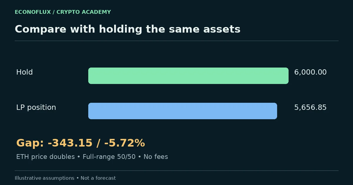
Now let ETH's external price double to 4,000 while the second asset retains its assumed value. In equilibrium, y divided by x must equal 4,000, while x times y remains 2,000. Solving gives approximately 0.707107 ETH and 2,828.427 units of the second asset. Their total value is about 5,656.85.
Holding the original one ETH and 2,000 units outside the pool would instead be worth 6,000. The difference is about 343.15, or 5.72% of the holding benchmark. The liquidity position gained approximately 41.42% from its original 4,000 value, but still underperformed holding by 5.72%. Both statements can be true simultaneously.
The formula and the assumptions it requires
For this specific full-range, fee-free, equal-value constant-product model, let r be the ratio of the new relative price to the original relative price. The liquidity-position value divided by the holding value is 2 times the square root of r, divided by 1 plus r. Subtract one to express the relative difference.
For r equal to two, the result is approximately negative 5.72%. For r equal to four, it is negative 20%. For r equal to one-half, it is again approximately negative 5.72%. The symmetry concerns a relative-price ratio, not identical cash outcomes. A decline in ETH can produce very different absolute portfolio value from a rise.
Do not apply this formula to a concentrated range, a weighted pool with different proportions or a stable-swap curve without checking the relevant model. A calculator that asks only for a price change may be silently assuming full-range 50/50 liquidity. Knowing the assumptions is more valuable than obtaining a precise-looking percentage from the wrong equation.
Why the word impermanent can mislead
In the idealized model, if the relative price returns exactly to its starting point while the position remains in place, the fee-free divergence disappears. That conditional possibility explains the name. It does not promise that prices will return, that the pool will survive or that you can wait without needing the funds.
Withdrawing while the ratio is different fixes the asset mix you receive at that moment. Future performance then depends on what you do with those assets. Calling the earlier gap impermanent does not make it economically irrelevant. It represents a genuine opportunity cost relative to holding the original portfolio.
In more complex strategies, rebalancing a concentrated position, changing ranges or repeatedly withdrawing can create a path-dependent result. Fees and losses accumulate over a sequence, not just at one final price ratio. A simple endpoint formula should not be used to reconstruct a strategy that changed its composition repeatedly.
Trading fees may offset divergence, but are uncertain
Liquidity providers may earn a share of trading fees according to the pool's rules. In the doubling example, fees and other net income would need to exceed the 343.15-unit gap to outperform the holding benchmark at that endpoint. This comparison should include the current value of the assets in which fees were earned and any costs of collecting them.
An advertised fee APR often extrapolates a recent period. Trading volume, active liquidity, fee settings and your position's share can change. A high historical rate does not guarantee enough future income to cover divergence. Incentive tokens add another price exposure and may have limited duration or become difficult to sell at the displayed valuation.
Avoid adding an APR percentage directly to an impermanent-loss percentage without matching denominators and time periods. One may be annualized relative to deposited capital, while the other is a point-in-time shortfall relative to holding. Calculate both portfolios in the same unit at the same endpoint, including actual fees and expenses.
Concentrated liquidity changes the analysis
Concentrated designs let providers choose a price range in which their liquidity is active. This can increase fee exposure per unit of deployed capital near the current price, but also changes the position's sensitivity. When price moves outside the chosen range, the position can become entirely one asset and stop earning trading fees until it becomes active again, depending on the protocol design.
A narrow range is therefore not simply a higher-yield version of the full-range example. It can require closer monitoring, more rebalancing and additional gas. The provider may repeatedly sell exposure to the asset that is rising or accumulate the asset that is falling. The full-range formula cannot capture those choices by itself.
Read how the specific protocol accounts for uncollected fees, range boundaries and liquidity changes. A management vault may automate the process but adds its own strategy, fee and contract risks. Automation does not remove the economic trade-off; it delegates decisions about how to manage it.
Similar asset prices do not eliminate risk
Pools pairing assets expected to track similar values can experience smaller relative-price changes during ordinary conditions. That observation does not guarantee small losses in stress. A stablecoin can lose its peg, a wrapped token can lose redeemability and a liquid-staking token can trade differently from its reference asset.
If traders exchange a deteriorating asset for the stronger one, the pool may accumulate the weaker asset. A history of stable relative prices can therefore be a poor guide to a rare but severe event. Ask what makes the assets track each other and what would happen if that mechanism failed.
These risks are separate from contract exploits, compromised administration, oracle failures or fraudulent tokens. Impermanent-loss calculations assume assets and contracts behave according to the model. They do not put a ceiling on total losses. A mathematically mild price scenario cannot establish that a pool is safe.
Build a decision worksheet before depositing
Record the exact pool, assets, fee tier, liquidity design and any chosen range. Write down the original quantities and their prices. Construct a holding benchmark that keeps those quantities unchanged. Then calculate the liquidity position under several relative-price scenarios, including a substantial move in either direction.
Add realistic costs and separate observed fee income from projected income. Show what happens if trading volume falls or incentives end. If you cannot reproduce the basic comparison, treat a dashboard's projected return as an unexplained estimate. A deposit should not be necessary to discover how the position works.
Use read-only views to inspect the intended contracts and route. Approvals, custody and exit procedures need their own review. Existing Academy guides cover those operational risks. This article's contribution is the benchmark calculation: it helps identify whether providing liquidity is actually doing better than keeping the same assets outside the pool.
Frequently asked questions
Can I make a cash profit and still have impermanent loss? Yes. The liquidity position can rise in value while rising less than the original assets held separately. The reference portfolio determines the relative loss.
Does withdrawing cause the loss? Withdrawal realizes a particular asset mix, but the divergence already exists in the position's economic value before withdrawal. Avoiding withdrawal does not guarantee recovery.
Will fees always compensate me? No. They depend on future trading and the pool's rules. Compare actual net income with the benchmark gap rather than relying on an advertised annual percentage.
Are stablecoin pools immune? No. Relative prices can diverge during a depeg, and contract or issuer risks remain even when prices appear stable. Similar prices are an assumption to investigate, not a guarantee.
Can I use the 50/50 formula for any pool? No. It applies to the stated full-range constant-product assumptions. Other weights, curves and concentrated ranges require their own calculations and documentation.
Sources & further reading
Sources and methodology · Report a correction
For information only. Not financial advice.